On October 6th, 2026, OpenAI released a repository containing 722 manuscripts that made progress on 373 open problems in mathematics, providing Lean proofs for many of them. The event, affectionately called the “slop drop” or “mathpocalypse”, has naturally caused quite the uproar in the mathematics community, but this post is not meant to delve into this controversy. This is just my attempt at digesting one of the results. I give some of my personal thoughts in the afterword.
In the repository, one proof shows that the matrix multiplication exponent over the complex numbers ωC is at most 9/4[1], and several preprints and Lean proofs that were posted soon after generalize the result to all fields [2][3][4][5]. This is a drastic improvement over the previous bound ω≤2.371177 due to Dupont et al. [6]. This marks the largest single improvement to the upper bound of ω since Schönhage in 1981 [7]. The methodology of this paper is also substantially different from that of the last 40 years of literature on the problem. In 1987, Strassen introduced the laser method for bounding ω[8], and until now, all of the improvements since then have been refinements of this method. The OpenAI proof instead leverages another idea Strassen introduced in 1988 called the asymptotic spectrum of tensors [9]. Remarkably, this proof gives a completely non-constructive bound on ω. It proves the existence of an O(n9/4+ε) matrix multiplication algorithm without describing one.1
None of the writing in this post was generated by LLMs, but they were used extensively to generate visuals, understand the proof, and simplify it to work over arbitrary fields. While prior knowledge of Strassen’s algorithm might be helpful, the technical parts of this post do not assume any familiarity with the theory of matrix multiplication, just basic field theory and tensors.
Matrix Multiplication as a Tensor Problem
Let F be a field.
Since the field is arbitrary and fixed, we use ω to mean ωF. We know ω≥2 because any algorithm must read its input, and the naive matrix multiplication algorithm gives ω≤3. It is widely believed that ω=2, but mathematicians have struggled to prove it for the better part of a century.
The first improvement on the naive bound was in 1969 due to Strassen [10]. He showed how to multiply two 2×2 matrices using only 7 multiplications instead of the naive algorithm’s 8. This generalizes to arbitrary matrices by treating this as a base case and recursively splitting the matrices into quadrants and multiplying them, only requiring 7 recursive calls. This algorithm proves ω≤log27≈2.807. More generally, if we can show that multiplying two n×n matrices requires no more than p multiplications, then ω≤lognp by a similar recursive algorithm. The following setup formalizes this idea of counting the number of multiplications.
Given two n×n matrices A,B∈Fn×n, their product C=AB satisfies
Cik=j∑AijBjk.
Let cij∈Fn×n be the matrix with a 1 in entry ji and 0 everywhere else (the indices switching is convenient for symmetry but otherwise unimportant). We are then trying to compute
Each of the 8 terms in this summation corresponds to one multiplication performed in the naive algorithm. However, Strassen’s algorithm gives a way to rewrite C with only 7 terms:
To be precise, each term represents one multiplication because it is the product of linear forms on the entries of A, the entries of B, and the matrices cij. Let aij,bij∈(Fn×n)∗ both be the map A↦Aij. We can write matrix multiplication as the bilinear map φn:Fn×n×Fn×n→Fn×n where
AB=φn(A,B)=i,j,k∑aij(A)bjk(B)cki.
So the minimum number of multiplications p required to multiply two n×n matrices is also the minimum value of p such that
φn(A,B)=i=1∑pui(A)vi(B)wi
where ui,vi∈(Fn×n)∗ and wi∈Fn×n. For vector spaces U,V,W, we can associate a bilinear map f:U×V→W with an order 3 tensor t∈U∗⊗V∗⊗W via the canonical isomorphism that sends the simple tensor u⊗v⊗w to the map (A,B)↦u(A)v(B)w. Under this isomorphism, φn is associated with
⟨n,n,n⟩=i,j,k∑aij⊗bjk⊗cki.
We call ⟨n,n,n⟩ the n×n matrix multiplication tensor. More generally, ⟨m,n,p⟩ is the tensor representing the multiplication of an m×n matrix by an n×p matrix. We call the three blocks of variables the legs of the tensor.
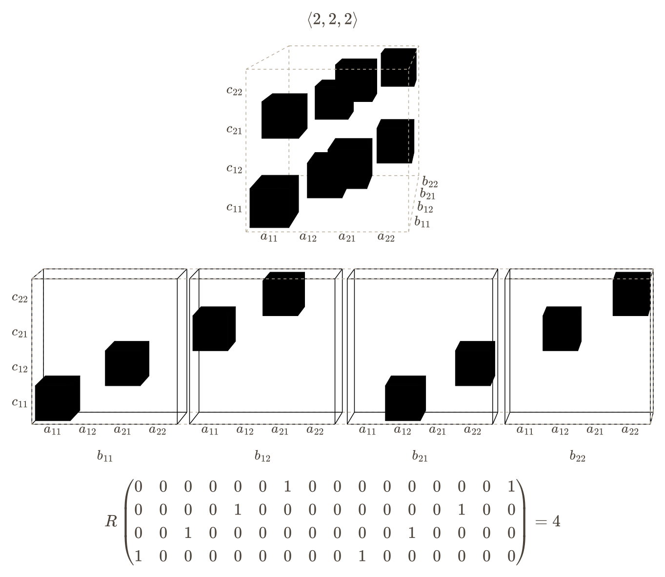
For example, we know R(⟨2,2,2⟩)≤7 by Strassen’s algorithm:
In fact, Winograd proved that R(⟨2,2,2⟩)=7[11]. Now we can state more concisely that the minimum number of multiplications required to multiply two n×n matrices is R(⟨n,n,n⟩).
This follows by using the rank decomposition of ⟨n,n,n⟩ as the base case for a recursive algorithm à la Strassen. It actually holds that ω=ν, but the other direction has a more involved proof and is not necessary for our purposes.
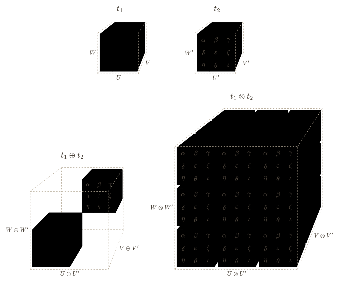
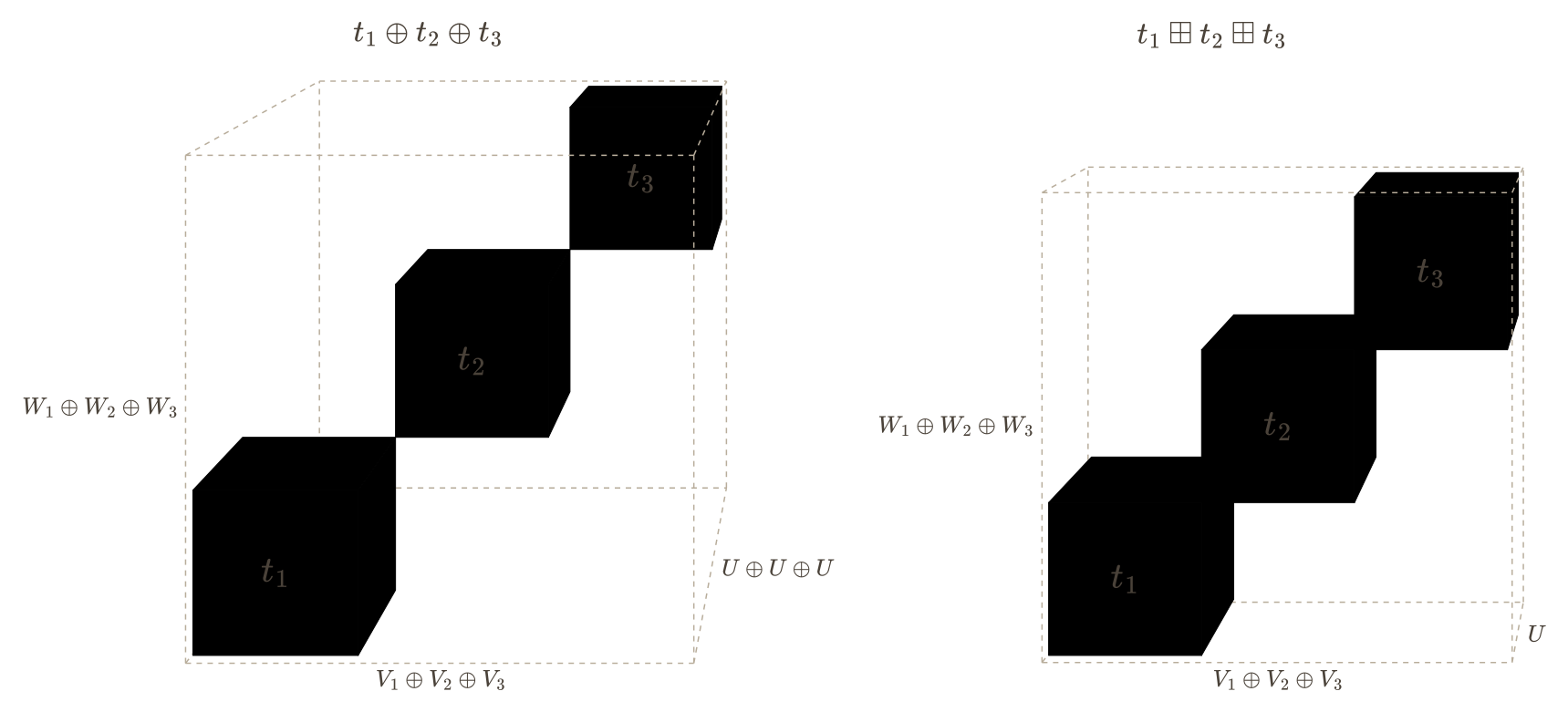
There are two primary operations of interest when working with tensors: the direct sum and the tensor product. If we picture a tensor in U⊗V⊗W as a cuboid of elements of F where each axis corresponds to a basis of U, V, or W, then these operations have nice visualizations.
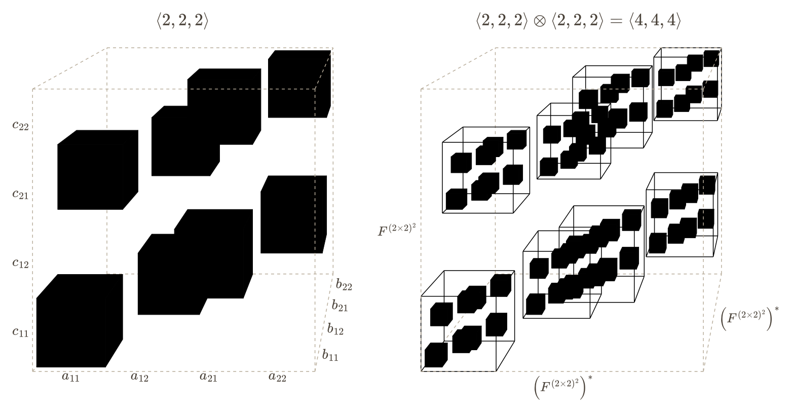
The following figure shows the recursive splitting of 4×4 matrices into quadrants to get ⟨2,2,2⟩⊗⟨2,2,2⟩=⟨4,4,4⟩. Each colored cube represents a coefficient of 1.
Let t1∈U⊗V⊗W and t2∈U′⊗V′⊗W′ be tensors.
We omit the proof because it is boring. Inconveniently, tensor rank is neither additive under direct sums nor multiplicative under tensor products. Strassen conjectured in 1973 that tensor rank was additive and it was not until 2019 that Shitov provided a counterexample [12]. The next section defines tools to get around this inconvenience.
The Asymptotic Spectrum of Tensors
First, we define a way to compare two tensors.
The simplest example of a restriction is t≥⟨0⟩ for all tensors t. Here, ⟨0⟩ is the zero tensor. Another example is that every nonzero tensor restricts to every simple tensor.
For an integer m>0, let ⟨m⟩∈Fm⊗Fm⊗Fm be the unit tensor. If ei∈Fm is the vector with a 1 in its i-th entry and 0 everywhere else, then
⟨m⟩=i=1∑mei⊗ei⊗ei.
We can also define the rank of a tensor in terms of restrictions.
This is true because picking m simple tensors ui⊗vi⊗wi that sum to t is equivalent to picking three linear maps rU,rV,rW under the correspondence
rU(ei)=ui,rV(ei)=vi,rW(ei)=wi.
The following proposition is another useful fact about restrictions.
This holds because we get a rank decomposition of t2 by applying rU⊗rV⊗rW to each term in a rank decomposition of t1.
Write t1∼t2 if t1 and t2 are restrictions of each other (i.e., t1≥t2 and t2≥t1). Note that ∼ is an equivalence relation. Let S be the commutative semiring (a ring that does not require additive inverses) of all three-legged tensors modulo ∼ under direct sum and tensor product. In this post, we use = on tensors to mean equality in S. We are now ready to define the object central to the main proof of the paper.
Instead of calling them tensor characters, Strassen used the name spectral points when he introduced them [9]. Like the tensor rank, a tensor character is a measure of the complexity of a tensor but with the benefit of being additive and multiplicative. The core idea of OpenAI’s proof is to make general statements about the entire asymptotic spectrum, not a particular character, and combine these statements with existing results connecting the asymptotic spectrum to the tensor rank. We begin to explore this relation with the following proposition.
The proof is short. Let m=R(t). By Proposition 6, ⟨m⟩≥t. Since ξ is monotone with respect to restriction,
ξ(⟨m⟩)≥ξ(t).(1)
But if we write ⟨m⟩=⟨1⟩⊕⋯⊕⟨1⟩, the additivity and unitality of ξ imply
As we learn more about tensor characters, it helps to have a concrete example in mind. The simplest example is called the flattening rank. To compute it, take a tensor in Fm⊗Fn⊗Fp, flatten it into a matrix Fm×np, and take its rank. This can be done along any of the three legs.
Next we study the value of tensor characters on matrix multiplication tensors. A useful fact is that
⟨m,n,p⟩⊗⟨m′,n′,p′⟩=⟨mm′,nn′,pp′⟩.
In particular, we can write
⟨n,n,n⟩=⟨n,1,1⟩⊗⟨1,n,1⟩⊗⟨1,1,n⟩.
We call these three factors the dot product tensors. The rank of these tensors is exactly n. The upper bound follows immediately from the naive matrix multiplication algorithm, and the lower bound can be shown using the flattening rank and Proposition 9. It happens that tensor characters are very well-behaved on dot product tensors.
We prove the claim for ℓ1(ξ) and the other two follow similarly. For concision, write ℓ1=ℓ1(ξ). First, we show an incorrect proof and then how to correct it. Set
ℓ1=log2ξ(⟨2,1,1⟩).
Then
nℓ1logn2=2ℓ1=ξ(⟨2,1,1⟩)=ξ(⟨nlogn2,1,1⟩).(3)
If we erroneously allow arbitrary positive real tensor powers instead of just integers, then
Taking the (logn2)-th root of (3) and (4) would finish the proof. To fix this argument, we rely on a common technique in the study of matrix multiplication: taking the limit of a large tensor power. We then combine this trick with the squeeze theorem. For p≥1, let s=⌊plog2n⌋:
We know ⟨n,n,n⟩≥⟨n⟩ by setting all the off-diagonal entries to 0, so ξ(⟨n,n,n⟩)≥n. This tells us L(ξ)≥1.
Approximate Algorithms
In 1980, Bini proved a key result that unlocked all of the improvements to ω that followed. Informally, it states that if there exists an efficient algorithm that approximates the product of two matrices, then there exists an exact algorithm whose asymptotic runtime is arbitrarily close to that of the approximate algorithm [13]. We now formalize what is meant by an approximate algorithm.
Let ∣∣⋅∣∣ be a norm on U′⊗V′⊗W′. We would like to say that t1 approximately restricts to t2 if for all ε>0, there exists a tensor e with ∣∣e∣∣<ε such that t1≥t2+e. Here, e represents some small error term. However, this sort of analytic definition does not generalize well to arbitrary fields where only the trivial metric might exist. Instead, we opt for a more algebraic definition.
So instead of adding a “small” tensor to t2, we use a function of some indeterminate ε. For convenience, this function is a polynomial. And while this is never explicitly performed, we can imagine scaling by ε−h and taking the limit as ε→0 to get t2. In this way, degeneration is the more general form of approximate restriction that we were looking for. Trivially, if t1≥t2, then t1⊵t2.
If allowing for a leading εh seems strange, note that the definition collapses to restriction if we require (dU⊗dV⊗dW)(t1)=t2+εe. This alternative equation can be satisfied for an equivalent definition if we also adjoin ε−1 to the codomains of dU,dV,dW, but this makes it more tedious to define the degree of degeneration.
In the style of Proposition 6, we define an approximate form of tensor rank in two ways.
Note that R(t)≤R(t) for all tensors t. Border rank behaves similarly to the regular tensor rank as in Proposition 4 and Proposition 7 with similarly routine proofs.
Now we can state the theorem that connects the border rank to exact algorithms.
This is exactly the statement from Proposition 3 but with the border rank instead of the regular tensor rank. The original theorem is slightly more general, considering rectangular matrix multiplication tensors instead of only square ones, but this is unimportant for our purposes. In fact, we do not need this theorem at all for the main proof. However, it is still valuable to show its proof because we will employ similar techniques later on.
We start with a lemma that tells us how to get from a degeneration to a restriction. Let t⊕k and t⊗k denote repeated direct sums and tensor products respectively.
Then t2 is the sum of the coefficients of terms with degree h:
t2=i+j+k=h∑(dU(i)⊗dV(j)⊗dW(k))(t1).
The number of triples (i,j,k)∈Z≥03 with i+j+k=h is exactly Nh=(2h+2).2
If we imagine each map in the sum being applied to a different copy of t1, we can rewrite the above equation as a function of t1⊕Nh. We index the components of this direct sum using triples (i,j,k). Let πU(i,j,k):U⊕Nh→U be the projection onto the (i,j,k)-th component, and similarly define πV(i,j,k) and πW(i,j,k). Let
The last step is to express this as a restriction map, meaning we need the tensor product of three homomorphisms, not the sum of many such tensor products. Luckily, we can take advantage of the fact that t1⊕Nh, when embedded in U⊕Nh⊗V⊕Nh⊗W⊕Nh, is only nonzero along the diagonal components U(i,j,k)⊗V(i,j,k)⊗W(i,j,k). So
It is not the case that the maps in (6) and (7) are the same. In general, sums and tensor products do not commute like this and (7) has many more terms than (6). But all of the new terms are only nonzero outside of the diagonal that t1⊕Nh occupies, so they evaluate to 0. This proves the lemma.
Now we prove Theorem 15. Suppose R(⟨n,n,n⟩)=m. By the definition of border rank, ⟨m⟩⊵⟨n,n,n⟩. Let h be the degree of degeneration. We again rely on analyzing a large tensor power, this time of ⟨n,n,n⟩. Observe that ⟨mp⟩⊵⟨n,n,n⟩⊗p with degree ph. By Lemma 16,
Since this holds for all p, we can take the limit as p→∞. The rightmost term above goes to 0 because Nph is a polynomial in p and grows slower than np, so
ω≤lognm=lognR(⟨n,n,n⟩).
This holds for all n, so reapplying the infimum finishes the proof.
We end the section by giving a name to the quantity that allowed us to prove the previous theorem.
Using the submultiplicativity of the tensor rank, we can apply Fekete’s lemma, a classical result from real analysis, to write
R(t)=p→∞limR(t⊗p)1/p.
To recap, we now have three variations on the idea of tensor rank that relate to each other as follows:
R(t)≤R(t)≤R(t).
And when applied to ⟨n,n,n⟩, they bound ω as in (8):
Taking the limit as p→∞ gives the desired result because Nph is a polynomial in p, meaning Nph1/p goes to 1.
Using this, we also get an analogue to Proposition 9 for the border rank whose proof is identical except that it substitutes degenerations for restrictions and border rank for the regular tensor rank.
The following is a foundational result in the study of asymptotic spectra due to Strassen [9]. This theorem is essential to the main argument of this post, but the proof is long so we refer the reader to the excellent exposition by Wigderson and Zuiddam, particularly Theorem 3.25 [14].
Polynomial Multiplication Tensors
Instead of directly analyzing matrix multiplication tensors, we study a closely related family of tensors: those representing polynomial multiplication. Let Pd be the vector space of polynomials with coefficients in F of degree at most d−1 with variable u. Let f∈Pa and g∈Pb be written as
f=i=0∑a−1αiui,g=j=0∑b−1βjuj.
Then their product is
fg=i=0∑a−1j=0∑b−1αiβjui+j.
Analogously to matrix multiplication, we can interpret polynomial multiplication between Pa and Pb as a bilinear map and associate it with a tensor C(a,b)∈Pa∗⊗Pb∗⊗Pa+b−1 where
C(a,b)=i=0∑a−1j=0∑b−1xi⊗yj⊗zi+j.
Here, xi(f)=αi, yj(g)=βj, and zk=uk. Observe that C(a,1)=⟨a,1,1⟩ and C(1,a)=⟨1,1,a⟩. This is the connection that allows us to derive statements about matrix multiplication from polynomial multiplication.
The reason it is helpful to study these tensors is that we know a lot more about them than matrix multiplication tensors.
This equality actually holds for the regular tensor rank when F has at least a+b−2 elements, but we do not need that.
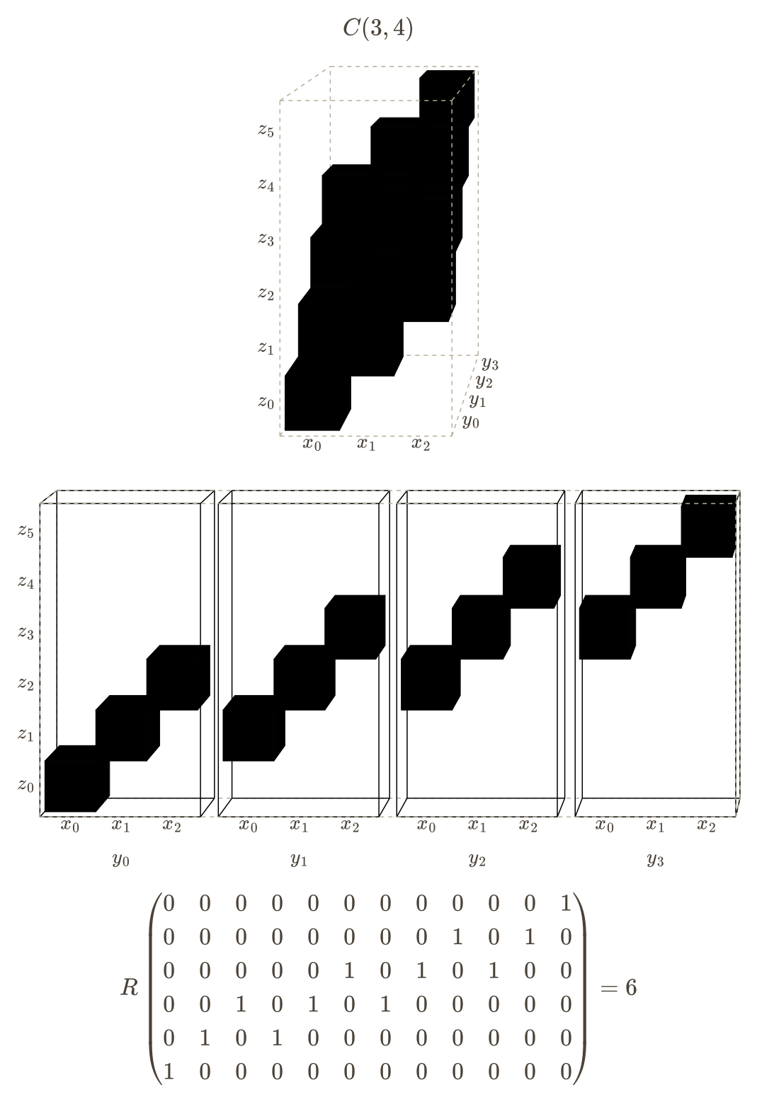
≥: By Corollary 19, the border rank is bounded from below by any tensor character, so we use the flattening rank on the third leg. This evaluates to a+b−1, and is illustrated below for C(3,4).
≤: Take f∈Pa and g∈Pb. Lagrange interpolation tells us that the product fg is entirely determined by its value at a+b−1 distinct points. However, F might not have that many elements, so consider the field F(ε). Importantly, this field is infinite even when F is finite. Interpret f and g as elements of the polynomial ring F(ε)[u]. Apply Lagrange interpolation with inputs ε1,…,εa+b−1 to write
Recall that F(ε) is the field of fractions of F[ε]. Let D∈F[ε] be the product of all the denominators of the Li and let c be the coefficient of the lowest degree term of D. So we have c−1DLi∈F[ε][u]. The maps x^i:f↦f(εi) and y^i:g↦g(εi) are linear forms over F[ε]. Thus,
c−1DC(a,b)=i=1∑a+b−1x^i⊗y^i⊗c−1DLi.
Since the lowest degree term of c−1D has coefficient 1, the left-hand side becomes εhC(a,b)+εh+1e for some e∈(Pa∗⊗Pb∗⊗Pa+b−1)[ε], precisely the definition of the border rank.
One minor inconvenience of the vocabulary we have built up so far is that it is sensitive to the order of the tensor legs. While U⊗V⊗W is trivially isomorphic to V⊗W⊗U, our notions of restriction, degeneration, and tensor characters do not recognize this. Define an action of the symmetric group S3 on the set of all three-legged tensors where σ∈S3 permutes the legs of the tensor it acts on. For example, if t∈U⊗V⊗W, then (321)t∈V⊗W⊗U. It will be convenient to have a function that behaves like a tensor character on polynomial multiplication tensors but is invariant under this action. For some ξ∈Δ(S), define Ξ:S→R≥0 such that
Ξ(t)=(σ∈S3∏ξ(σt))1/(2L(ξ))
where L(ξ) is defined as in Corollary 11. This function is monotone with respect to restriction and degeneration, multiplicative under tensor products, and interestingly superadditive under direct sums (more on that later). For concision, let γ(a,b)=Ξ(C(a,b)). In addition to being symmetric with γ(a,b)=γ(b,a), this function was selected to have the convenient property that γ(1,b)=b, which follows from Proposition 10. By Corollary 19 and Proposition 21, ξ(C(a,b))≤a+b−1, so
γ(a,b)≤(a+b−1)3/L(ξ).(10)
Main Theorem
We work backwards from the result.
It turns out that this theorem follows quickly from a lower bound on the diagonal of γ.
So now we need to prove Lemma 23, which we will do using two more lemmas whose proofs we defer to the following sections.
For a visual aid, note that f(x,y)=xy also satisfies both lemmas.
The proof of Lemma 23 does not rely on anything related to tensor characters and only uses the two lemmas above. Intuitively, Lemma 25 gives us a lower bound on the growth of γ between (a,b) and (a,3b+a−1), but Lemma 24 tells us that γ grows more slowly as its coordinates increase, meaning most of that growth is happening near (a,b). We apply this to the case a=b to lower bound the diagonal of γ. Let
δ(a,b)=γ(a,b+1)−γ(a,b).
By Lemma 24, δ is nonincreasing in b. Use this and Lemma 25 to write
This is a telescoping product that evaluates to a4/3, proving the lemma.
Shared-Leg Sums
This section is where this post diverges from the original proof. The OpenAI preprint relies on the existence of roots of unity to prove its Proposition 3.1, but their use is superficial and the proof is simpler without them. We demonstrate this in Proposition 27, generalizing the argument to work over all fields. Then their Corollary 3.2 has an unnecessarily convoluted statement of which we give an alternative in Lemma 28 that is easier to describe.3
Dot product tensors are a key ingredient in the main proof, so it is helpful to study tensor products of the form t⊗⟨1,1,n⟩. Recall
⟨1,1,n⟩=C(1,n)=i=1∑nx⊗yi⊗zi.
So the first leg of t⊗⟨1,1,n⟩ is the same as the first leg of t, and the second and third legs are n disjoint copies of the second and third legs t. More generally, we can define this operation of taking a direct sum where the first leg is shared.
Using this notation, we can write more concisely
t⊗⟨1,1,n⟩=t⊞n.
While this operation arises naturally when working with polynomial multiplication tensors, it does not keep the nice properties that direct sums have. In particular, tensor characters are not additive under shared-leg sums. Trivially, t1⊕t2≥t1⊞t2, so
ξ(t1⊞t2)≤ξ(t1⊕t2)=ξ(t1)+ξ(t2),
giving us only subadditivity. The following proposition is the key degeneration that allows us to also compute lower bounds on the tensor characters of shared-leg sums, transforming shared-leg sums into direct sums.
where ui′,vj′(k),wk′(k) are basis elements of U,Vk,Wk respectively. Consider the terms with i=k. If we associate each xk⊗ui′ with a basis element x0⊗ui′(k)∈P1∗⊗Ua, then these terms look like
Up to reindexing the z variables, these are exactly the terms of C(1,a)⊗(t0⊕⋯⊕ta−1). So we need to define the degeneration to eliminate all terms with i=k. Intuitively, we are giving up the first input of C(a,a) in exchange for separating the first legs of all the ti. Define
This expression is minimized when i=k, so we keep only the desired terms. Note that the 4a2 term is only there to keep the exponent of ε in dW positive.
Using this degeneration, we can prove a very useful property about Ξ.
The proof borrows techniques from the laser method introduced by Strassen [8]. Let t=(t0⊞t1)⊗p be a large tensor power, which is an element of U⊗p⊗(V0⊕V1)⊗p⊗(W0⊕W1)⊗p. Our goal is to degenerate t to a direct sum instead of a shared-leg sum in order to take advantage of the additivity of tensor characters. Every basis element in the second leg lives in VB1⊗⋯⊗VBp for some binary string B∈{0,1}p, and similarly every basis element in the third leg lives in some WB1⊗⋯⊗WBp. Write these spaces as VB and WB for short. Tensor products distribute over shared-leg sums, so we can also write
t=B∈{0,1}p⊞(tB1⊗⋯⊗tBp)=B∈{0,1}p⊞tB.
For an integer k0≥0, let K be the set of all binary strings with exactly k0 zeros. We restrict t by zeroing every basis element in the second and third legs that is not in VB or WB for some B∈K. What we are left with is
t≥B∈K⊞tB.
Call the shared-leg sum on the right-hand side above s. When considered individually, each term of s is equal to t0⊗k0⊗t1⊗(p−k0). It is tempting to say s=⟨1,1,∣K∣⟩⊗t0⊗k0⊗t1⊗(p−k0), but this is incorrect, and this statement still would not be true if the equality were replaced by a restriction in either direction (finding explicit counterexamples is somewhat involved). The first legs of the summands interact with each other, so we need to apply Proposition 27 to obtain a direct sum:
As p→∞, the denominator approaches 1, finishing the proof.
Concavity
This section is dedicated to proving Lemma 24. The original preprint rushed through this proof and provided little motivation, so it took me by far the longest to comprehend. I want to highlight that this and the following sections follow the same pattern as the proof of the superadditivity of Ξ: Come up with a clever degeneration that looks similar to the inequality you are trying to prove, and then apply Ξ to both sides and use its monotonicity. First, we construct the degeneration in the following proposition.
Recall C(1,2)=⟨1,1,2⟩, so the presence of the shared-leg sum should not be surprising. And the statement of this proposition bears a striking resemblance to the statement of Lemma 24 when rearranged:
2γ(a,b)≥γ(a,b−1)+γ(a,b+1).(13)
Under the canonical isomorphism introduced in the beginning of the post, the tensor C(a,b)⊗C(1,2) corresponds to a bilinear map
μ:Pa×(Pb⊗P2)→(Pa+b−1⊗P2)
that maps (f,g)↦fg. Say P2 has variable v and all the other spaces have variable u, so here g is a polynomial in u and v whose degree in u is at most b−1 and whose degree in v is at most 1. Alternatively, think of g as a vector of length two with entries in Pb. We know there exists an isomorphism φd:Pd⊗P2→Pd−1⊕Pd+1 since they are both 2d-dimensional vector spaces over F. Let θ:Pa×(Pb−1⊕Pb+1)→Pa+b−2⊕Pa+b be the bilinear map associated with the shared-leg sum C(a,b−1)⊞C(a,b+1), the target of our degeneration. It maps (f,(g,h))↦(fg,fh). This gives us a square:
If this diagram were commutative, then the proof would be finished. In fact, we would have proved the stronger statement that the two tensors of interest are equal because their associated maps μ and θ would be the same up to isomorphisms on their outputs and second inputs. However, this is not generally the case. Instead, we will define φd in such a way that the diagram almost commutes, and use a degeneration to handle the error terms.
We construct φd by defining a basis Bd of Pd⊗P2 composed of two disjoint sets Bd− and Bd+ such that φd isomorphically maps Bd− onto Pd−1⊕0 and Bd+ onto 0⊕Pd+1. Let
Bd−={ui(u−v)∣0≤i<d−1},Bd+={uiv∣0≤i<d}∪{1}.
Indeed, these sets are disjoint, ∣Bd−∣=d−1, and ∣Bd+∣=d+1, so the dimensions are correct. They also span Pd⊗P2 because Bd+ contains 1 and every uiv, and the identity ui+1=ui(u−v)+uiv recovers the remaining monomials. Now that we have a basis, let
Take an arbitrary f∈Pa and write f=∑j=0a−1αjuj. Observe how on the second component, φd substitutes v↦u, an operation that commutes with multiplication by f. But on the first component, φd drops constant terms and divides by u−v. This does not commute with multiplication by f as we are about to see. We compute the values of φa+b−1∘μ when f is paired with each element of Bb:
In the first and second lines of each table, φa+b−1∘μ behaves identically to θ∘(idPa×φb). It is only on the third lines when the second input is 1 that they differ because φa+b−1 picks up some unwanted terms in the first component of the output. This is the noncommutativity of dropping constants mentioned above. We can get rid of that ∑j=1a−1αjuj−1 by using a degeneration to multiply it by a power of ε. First, we use (14) to see which components of the output are nonzero in the image of φa+b−1∘μ when the second input is restricted to Bb− or Bb+:
second inputBb−Bb+Pa+b−2outputPa+b−2✓✓Pa+b−2Pa+b×✓
The unwanted terms all live in the bottom-left entry, so if we imagine multiplying the second row and the first column each by ε, then the unwanted terms get multiplied by ε2 while the diagonal terms only get multiplied by ε (the top-right entry is empty so we ignore it). To formalize this, the degeneration needs three homomorphisms
Let dU be the identity. Multiplying the second row by ε means letting dV multiply the duals of elements of Bb+ by ε and then applying (φb−1)∗. Similarly, multiplying the first column by ε means letting dW multiply elements of Ba+b−1− by ε and then applying φa+b−1. Let ρ be the bilinear map associated with (dU⊗dV⊗dW)(C(a,b)⊗C(1,2)). So
where the first inequality is given by Proposition 29 and monotonicity, and the second inequality is given by superadditivity. Combining (15) and (16) proves the lemma as rearranged in (13).
Shifted Tripling
We are barreling down the home stretch and all that stands in our way is the following degeneration that enables us to prove Lemma 25.
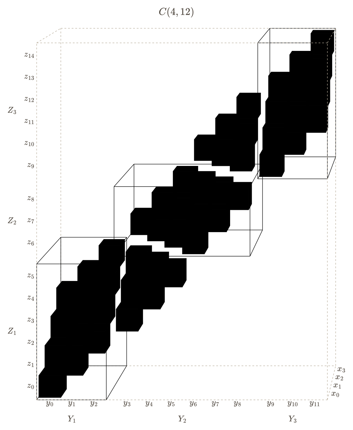
Partition each of the second and third legs of C(a,3b+a−1) into three parts as follows:
Consider only the terms in C(a,3b+a−1) whose variables in the second and third legs are from Yi and Zi respectively. When i is 1 or 3, we get a copy of C(a,b). When i=2, we get a copy of C(a,b) with the second and third legs swapped. The proofs of these equivalences are formal and involve a lot of tedious reindexing, so we omit them.
Our goal is to eliminate all terms with variables from Yi and Zj with i=j. Since every term is of the form xi⊗yj⊗zi+j and i<a, there are already no terms from the following pairs of blocks: (Y1,Z2),(Y1,Z3),(Y3,Z1),(Y3,Z2). So we only need to worry about Y2 mixing with Z1 and Z3. Let the degeneration maps multiply variables in Y2, Z1, and Z3 by ε. This multiplies all the unwanted terms by ε2 while all the other nonzero terms only get multiplied by ε, giving us the desired result. The following figure shows this degeneration with a=4 and b=3.
Lemma 25 follows immediately by applying Ξ and its superadditivity to both sides of this degeneration.
Afterword
As I was working on this post, especially toward the end, I kept questioning myself: “Why am I writing this?” What is the purpose of repackaging AI-generated math? The reason I had when I started was simple. I wanted to create a learning resource accessible to math and computer science undergraduates that consolidated into one place everything you needed to understand the newest developments in the theory of matrix multiplication. I started learning about this subject almost two years ago, before LLMs took math by storm, because I read in Yufei Zhao’s excellent Graph Theory and Additive Combinatorics that the existence of large sets with no three-term arithmetic progressions given by Behrend’s construction was an integral part of Coppersmith and Winograd’s matrix multiplication algorithm [15][16]. Put simply, a clever construction in combinatorics somehow enabled progress to be made on the upper bound of ω. This was such a surprising connection to me and I desperately wanted to understand it. I found myself bouncing between many learning resources, the most helpful of which was probably Williams’ lecture notes, until I eventually wrapped my head around the proof. I then started working on a video for my YouTube channel explaining the main ideas of the argument, but the project quickly grew in scope and I had to put it on the back burner.
Cut to October 6th when I found out OpenAI released a proof that ω≤9/4. I opened the preprint and was shocked at how short it was: only 13 pages with citations. Then I started reading it and was shocked again at how graspable many of the ideas were. Then I continued reading it and was not shocked at all when I realized many of the proofs were poorly written and that I was totally lost. So I set myself the goal to fully understand the paper and to write a post about it. I wanted to give the reader all the context they would need and to write the proofs in a simpler, more accessible way. It felt like I could produce something “useful”.
Now it is today, I am procrastinating on writing the last few proofs, staring at this blog post that has slowly ballooned into a textbook chapter, and I have had plenty of time to ruminate. What I have come to realize is that I have a second, more personal reason for writing this: This post is a certificate of my understanding. Sure, maybe I can save someone a few tokens who wants to learn about matrix multiplication, or maybe I can even introduce someone to the field (and I really hope I do!), but these hopes are tied to the vicissitudes of AI and how people spend their time. All that I can be truly certain of is that I, at this very moment, understand a proof that ω≤9/4. I am shouting into the void, “I get it!” That is inalienable.
Before finally signing off, I want to emphasize that this post was a lot of fun to write. I truly believe that this is one of the most exciting times to be a recreational mathematician. The barrier to engage with research mathematics has never felt lower, and I hope we continue to take advantage of that.
Footnotes
The reason ε needs to be in the time complexity is that ω is actually a limit point. Coppersmith and Winograd proved the surprising result that given an algorithm for multiplying matrices, there exists a faster one [17]. ↩
It feels strange to criticize the source material in this way, but I think this will become a more common practice in the brave new world. If exposition is going to play such an important part in the act of the doing mathematics, then highlighting the expository choices made should be an expected part of mathematical writing. On the other hand, I cannot help but worry that this sentiment might be a reflection of the current transitory state where LLMs are better provers but worse explainers and theory builders than humans. Maybe all that we will have left is the interpersonal: teacher empathizing with student, or colleague sharing with colleague. ↩
References
OpenAI. An Upper Bound of 9/4 for the Matrix Multiplication Exponent. OpenAI Math Release preprint https://github.com/openai/math/blob/main/preprints/Matrix-Multiplication-Nine-Fourths-October-2-2026/paper.pdf; 2026.
Lü H. Polynomial Separation of a Shared Tensor Leg and Matrix Multiplication in Arbitrary Characteristic. arXiv preprint arXiv:261018914. 2026;
Amanov A, Berg M van den, Zuiddam J. Multiplying matrices via polynomials: exposition and barriers. arXiv preprint arXiv:261030054. 2026;
Navot S. The Matrix Multiplication Bound ω≤9/4 over Arbitrary Fields [Internet]. Manuscript, GitHub repository selanavot/matrix-multiplication-all-fields; 2026. Available from: https://github.com/selanavot/matrix-multiplication-all-fields/blob/main/paper/paper.pdf
Zuiddam J. omega-nine-quarters-all-fields: Lean proof that the matrix multiplication exponent is at most 9/4 over every field [Internet]. GitHub repository; 2026. Available from: https://github.com/jzuiddam/omega-nine-quarters-all-fields
Dupont E, Eisenberger M, Kozlovskii B, Mehrabian A, Ruiz FJ, See A, et al. Improving the matrix multiplication exponent with modern optimization and AlphaEvolve. arXiv preprint arXiv:260816884. 2026;
Schönhage A. Partial and total matrix multiplication. SIAM Journal on Computing. 1981;10(3):434–55.
Strassen V. Relative bilinear complexity and matrix multiplication. 1987;
Strassen V. The asymptotic spectrum of tensors. 1988;
Strassen V. Gaussian elimination is not optimal. Numerische Mathematik. 1969;13(4):354–6.
Winograd S. On multiplication of 2×2 matrices. Linear algebra and its applications. 1971;
Shitov Y. Counterexamples to Strassen’s direct sum conjecture. 2019;
Bini D. Relations between exact and approximate bilinear algorithms. Applications. Calcolo. 1980;17(1):87–97.
Wigderson A, Zuiddam J. Asymptotic spectra: Theory, applications and extensions. Manuscript dated October. 2023;24.
Zhao Y. Graph theory and additive combinatorics: exploring structure and randomness. Cambridge University Press; 2023.
Coppersmith D, Winograd S. Matrix multiplication via arithmetic progressions. In: Proceedings of the nineteenth annual ACM symposium on Theory of computing. 1987. p. 1–6.
Coppersmith D, Winograd S. On the asymptotic complexity of matrix multiplication. SIAM Journal on Computing. 1982;11(3):472–92.